What is Fluorescence Lifetime?
The fluorescence lifetime (τ) is defined as the average time that a molecule remains in an excited state prior to returning to the ground state. For a single exponential decay, the fluorescence intensity as a function of time after a brief pulse of excitation light is described as
I (t) = I0 exp (-t/τ)
where I0 is the initial intensity immediately after the excitation pulse.
In practice, the fluorescence lifetime (τ-tau) is defined as the time in which the fluorescence intensity decays to 1/e of the intensity immediately following excitation. Fluorescence decay is often multiexponential, leading to complex decay curves.
Instrumental methods for measuring fluorescence lifetimes are divided into two major categories, frequency-domain and time-domain. Frequency-domain fluorometers excite the fluorescence with light, which is sinusoidal and modulated at radio frequencies (for nanosecond decays), and then measure the phase shift and amplitude attenuation of the fluorescence emission relative to the phase and amplitude of the exciting light. Thus, each lifetime value will cause a specific phase shift and attenuation at a given frequency.
In time-domain methods, pulsed light is used as the excitation source, and fluorescence lifetimes are measured from the fluorescence signal directly or by photon counting.
What is FLIM?
Many currently available fluorescence microscopic techniques, such as confocal or multi-photon excitation, cannot provide detailed information about the organization and dynamics of complex cellular structures. In contrast, time-resolved fluorescence microscopy allows the measurement of dynamic events at very high temporal resolution and can monitor interactions between cellular components with very high spatial resolution as well. Fluorescence lifetime imaging microscopy (FLIM) was developed to obtain a spatial and temporal distribution of molecular lifetime in a single living cell instead of decay curves only. Both time and frequency domain FLIM imaging systems are available on the market.
FLIM-FRET
The combination of lifetime and FRET (FLIM-FRET) provides high spatial (nanometer) and temporal (nanoseconds) resolution (Bacskai et al., 2003; Elnagovan et al., 2002; Krishnan et al., 2003). The presence of acceptor molecules within the local environment of the donor that permits energy transfer will influence the fluorescence lifetime of the donor. By measuring the donor lifetime in the presence and the absence of acceptor one can estimate the distance between the donor- and acceptor-labeled proteins. While 1p-FRET produces 'apparent' E%, i.e. efficiency calculated on the basis of all donors (FRET and non-FRET), the double-label lifetime data in 2p-FLIM-FRET usually exhibits two donor lifetimes (FRET and non-FRET), allowing to estimate the distance.
The energy transfer efficiency (E), the rate of energy transfer (kT), and the distance between the donor and acceptor molecules (r) are calculated using the following equations (Lakowicz, 1999):
where τD and τDA is the donor excited state lifetime in the absence and presence of the acceptor; R0 is the Förster distance -- that is, the distance between the donor and the acceptor at which half the excitation energy of the donor is transferred to the acceptor while the other half is dissipated by all other processes , including light emission; n is the refractive index; QD is the quantum yield of the donor; ĸ2 is a factor describing the relative dipole orientation (normally assumed to be 2/3 - Lakowicz, 1999).
Acquisition of FLIM - FRET Images
We use 2P FLIM-FRET Microscopy System to collect FLIM and FRET Images. Any fluorescence imaging requires careful selection of excitation power at the specimen plane in order to reduce photobleaching on one hand, but on the other hand reasonable photon counts in the acquired data to obtain a good statistical fit. We used unfused cells to obtain multiphoton excitation intensity spectra for CFP or Cerulean, YFP or Venus, GFP, BFP and dsRED within the ti:sapphire laser tuning range from 700-1000 nm. We selected the peak excitation wavelength from these spectra to excite fused and unfused cells of the above-mentioned GFPs for FLIM images and the lifetime numbers were measured using the lifetime data processing software (SPCImage; Becker & Hickl) at every pixel.
This FLIM imaging methodology acquired lifetime images of Cerulean-C/EBPα (donor) in the absence and presence of the acceptor Venus-C/EBPα. Mouse pituitary GHFT1-5 cells expressing Cerulean-C/EBPα alone (i.e. donor alone) were identified using an arc lamp light source. As described above, the 820 nm laser line was used as an excitation wavelength to illuminate the cell and the SPC-730 board was used to acquire lifetime images using 480/30 nm emission filters. The FLIM PMT was synchronized (see explanation in the Facilities Section) to the excitation laser pulse. The accumulation time was few seconds to obtain reasonable photon counts. The acquisition time varies depending on the expression of the fluorophores. The acquired image was processed using the SPCImage software to obtain the exponential decays of FRET-FLIM image.
We next imaged cells expressing the double-label combination of Cerulean-C/EBPα and Venus-C/EBPα (i.e. donor in the presence of the acceptor). The lifetime images were acquired using the same excitation (820 nm laser line) and emission filter (480/30 nm) used for donor alone lifetime image acquisition (www.chromatech.com). The double exponential fluorescence lifetimes were processed and calculated. Both sets of images (tD and tDA1, tDA2 were processed for lifetime FRET images. All images were acquired at room temperature (74oF). We did not observe any detectable autofluorescence signals using the unlabeled cells in the same media used for FRET-FLIM imaging.
Read our FLIM protocol published in Nature Protocol 2011.
Sample Images
Image
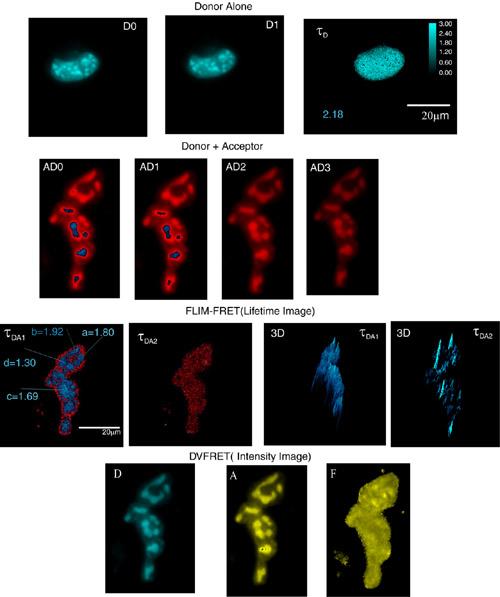
FLIM-FRET imaging of GHFT1-5 cells expressing BFP- and RFP-C/EBP. Time-resolved donor images were acquired in the presence (AD0, AD1, AD2, AD3, AD4) and absence (DD0, DD1) of the acceptor, and then processed. In the absence of the acceptor, one obtains donor (BFP-C/EBP) two-dimensional distribution of a single component lifetime image (D = 3.7 ns, at position '-c') and there is no 2nd component. But, in the presence of the acceptor (BFP-RFP-C/EBP), the processed images provide two-dimensional distributions of double component lifetime images (DA1 = 2.1 ns and DA2 = 0.78 ns, at position '-c'), indicating the occurrence of protein dimerization (DA1 < D) and distance distribution. Intensity FRET image (A/D = F) using DVFRET system were also acquired and processed for the same cell in a different system configuration, as explained in the text. As shown, the intensity FRET image (F) does not provide any detailed information regarding the energy transfer process. *DA1 is the same image DA1. Adapted from Periasamy et al., 2001, Methods in Cellular Imaging, edited by A. Periasamy, Oxford University Press, New York.